EN Medical device for dental professionals, clean and cold-sterilize before use. BG Медицинско изделие за специалисти по дентална медицина, почистете и стерилизирайте на студено преди употреба. CZ Zdravotnický prostředek určený pro zubní lékaře; před použitím jej vyčistěte a sterilizujte netermální metodou. DA Medicinsk udstyr til tandlæger og tandplejere. Rengøres og koldsteriliseres inden brug. DE Medizinprodukt für zahnmedizinisches Fachpersonal. Vor Gebrauch reinigen und kalt sterilisieren. EL Ιατροτεχνολογικό προϊόν για επαγγελματίες οδοντιάτρους. Να αποστειρώνεται εν ψυχρώ πριν από τη χρήση. ES Dispositivo médico para profesionales de la odontología; limpiar y esterilizar en frío antes de su uso. ET Hambaravispetsialistidele ette nähtud meditsiiniseade, puhastage ja külmsteriliseerige enne kasutamist. FI Hammaslääketieteen ammattilaisille tarkoitettu lääkinnällinen laite, puhdistettava ja kylmästeriloitava ennen käyttöä. FR Dispositif medical destiné aux professionnels dentaires, à nettoyer et stériliser à froid avant utilisation. HR Medicinsko sredstvo za stomatološke stručnjake, očistitii hladno sterilizirati prije uporabe. HU Orvostechnikai eszköz fogászatiszakemberek számára, használat előtt tisztítandó és hideg sterilizálással fertőtlenítendő. IT Dispositivo medico per personale odontoiatrico qualificato. Pulire e sterilizzare a freddo prima dell'uso. LT Gydytojams odontologams skirta medicinos priemonė. Prieš naudojant nuvalyti ir sterilizuoti žemoje temperatūroje.LV Medicīniska ierīce zobārstniecības speciālistiem. Pirms lietošanas notīrīt un veikt auksto sterilizāciju. NO Medisinsk utstyr for tannhelsepersonell. Rengjør og kaldsteriliser før bruk. NL Medisch apparaat voor tandheelkundige professionals, reinigen en koud steriliseren voor gebruik. PL Wyrób medyczny dla stomatologów, wyczyścić i wysterylizować na zimno przed użyciem. PT Dispositivo médico para profissionais de medicina dentária, limpar e esterilizar a frio antes de usar. RO Dispozitiv medical pentru stomatologi și asistenți de medicină dentară, a se curăța și steriliza la rece înainte de utilizare. SK Zdravotnícka pomôcka pre zubárov, pred použitím ju vyčistite a sterilizujte za studena. SL Medicinski pripomoček za zobozdravnike; pred uporabo očistite in hladno sterilizirajte. SV Medicinteknisk produkt för tandvårdspersonal, rengör och kallsterilisera före användning.
EN Assortment BG Артикул HR Asortiman CS Souprava DA Sortiment NL Assortiment ET Valik FI Lajitelma FR Assortiment DE Sortiment EL Συνδυασμός HU Készlet IT Assortimento LV Sortiments LT Asortimentas PL Asortyment PT Conjunto RO Set SK Zaradenie SL Asortiman ES Surtido SV Sortiment
EN (30 x each type) BG (30 x всеки тип) HR (30 x svaka vrsta) CS (každý typ 30×) DA (30 x hver type) NL (30 stuks per type) ET (30 × iga tüüpi) FI (30 kpl/malli) FR (30 unités/taille) DE (30 St./Größe) EL (30 τεμ. από κάθε τύπο) HU (30 db minden típusból) IT (30 pz/misura) LV (30 gab. no katra veida) LT (30 kiekvieno tipo vnt.) PL (30 x każdy rodzaj) PT (30 x cada tipo) RO (30 x fiecare tip) SK (30 x každý typ) SL (30 kosov vsake vrste) ES (30 unidades/tamaño) SV (30 st. / storlek)
Made in Finland
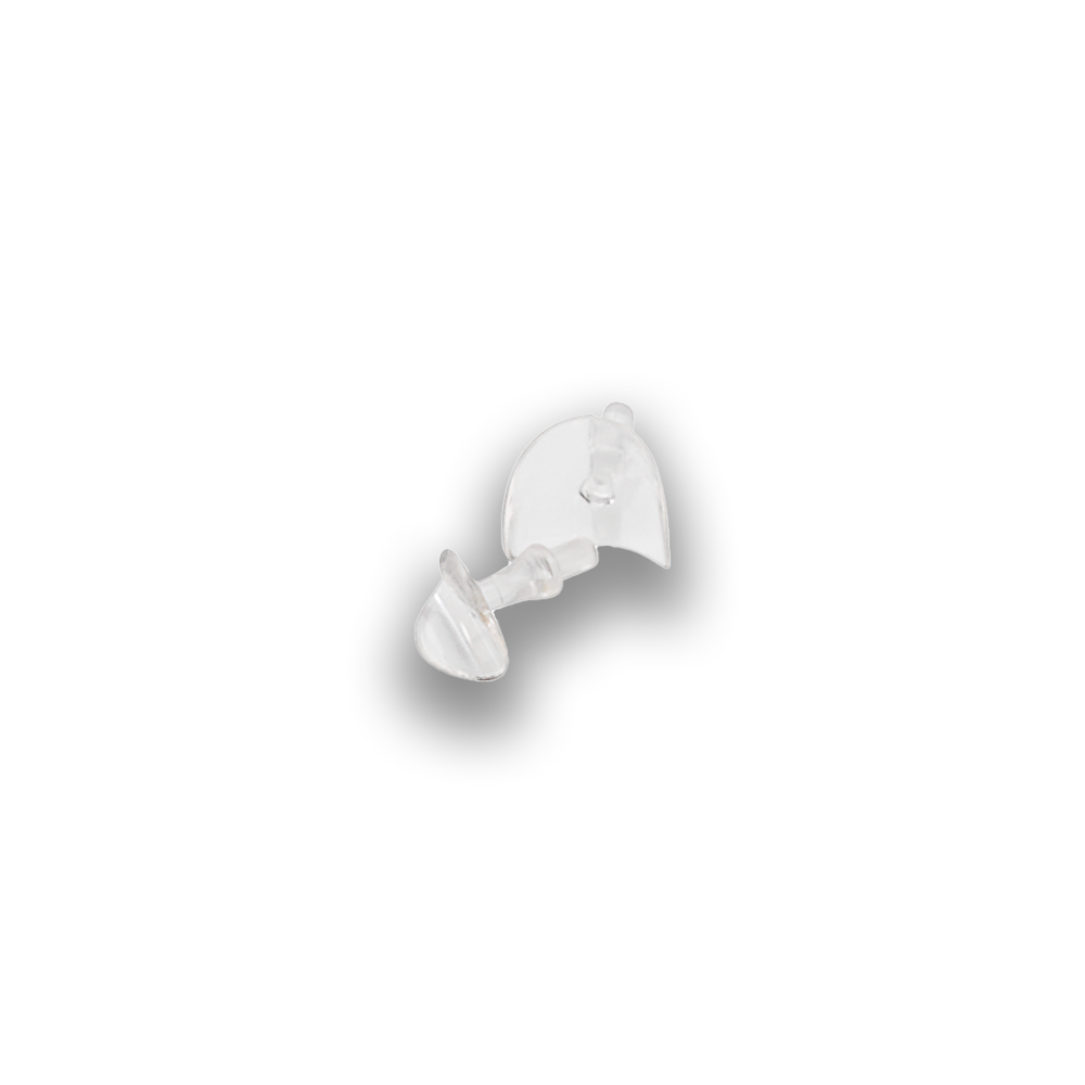
EN Reuse of this product may cause it to break, potentially compromising patient safety. Cervical matrices are of a flexible durable plastic and are disposable. Matrices can be cold-sterilized. The matrix can be formed and bent with pliers and scissors. For the removal of plastic working end we recommend LM-MultiLever™ (LM 7550). BG Повторната употреба на този продукт може да доведе до счупване, което може да застраши безопасността на пациента. Цервикални матрици са изработени от гъвкава пластмаса и са за еднократна употреба. Матриците могат да бъдат студено стерилизирани. Матриците могат да бъдат оформени и огънати с клещи и ножици. За отстраняване на пластмасовия работен край препоръчваме LM-MultiLever™ (LM 7550). HR Ponovnim korištenjem ovog proizvoda može doći do lomljenja,čime se potencijalno ugrožava sigurnost pacijenta. Cervikalne matrice napravljene su od fleksibilne plastike i jednokratne su. Matrice se mogu podvrgnuti hladnoj sterilizaciji. Matrica se može oblikovati i savijati s pomoću kliješta ili škara. Za uklanjanje plastičnog radnog dijela preporučujemo uporabu instrumenta LM-MultiLever™ (LM 7550). CS Při opakovaném používání se tento výrobek může poškodit, což může ohrozit pacienta. Krčkové matrice jsou vyrobené z pružného plastu a jsou jednorázové. Matrice je možné sterilizovat za studena. Matrici lze formovat a ohýbat kleštěmi a nůžkami. K vyjmutí plastového pracovního konce doporučujeme použít nástroj LM-MultiLever™ (LM 7550). DA Genbrug af dette produkt kan resultere i, at det brækker, hvilket potentielt kan udgøre en risiko for patientsikkerheden. Cervikal-matricer er fremstillet af fleksibelt plastik og er til engangsbrug. Matricerne kan koldsteriliseres. Matricen kan formes og bøjes med tænger og sakse. Til at fjerne arbejdsenden af plastik anbefaler vi LM-MultiLever™ (LM 7550). NL Bij hergebruik van dit product kan het stukgaan, wat de veiligheid van de patiënt in gevaar kan brengen. Cervicale matrices zijn gemaakt van flexibel plastic en bedoeld voor eenmalig gebruik. De matrices zijn geschikt voor koude sterilisatie. De matrix kan worden gevormd en gebogen met een tang en schaar. We raden aan de LM-MultiLever™ (LM 7550) te gebruiken om het plastic uiteinde te verwijderen. ET Toote korduskasutamine võib põhjustada selle purunemise ja ohustada patsienti. Tservikaalmaatriksid on valmistatud painduvast plastist ja on ühekordselt kasutatavad. Maatrikseid saab külmsteriliseerida. Maatriksit saab vormida ja painutada näpitsate ja kääride abil. Plastist tööotsaku eemaldamiseks soovitame kasutada toodet LM-MultiLever™ (LM 7550). FI Tuotteen uudelleenkäyttö saattaa aiheuttaa tuotteen rikkoutumisen, jolloin potilaan turvallisuus voi vaarantua. Kervikaalimatriisit on valmistettu joustavasta kestävästä muovista ja ne ovat kertakäyttöisiä; voidaan kylmästeriloida. Matriisia voi muotoilla ja taivuttaa käyttäen apuna pihtejä ja saksia. Suosittelemme muovikärjen poistamiseen LM-MultiLeveriä™ (LM 7550). FR Réutiliser ce produit risque de le briser et éventuellement de compromettre la sécurité du patient. Les matrices cervicales sont à usage unique et fabriquées en plastique résistant flexible. Les matrices cervicales peuvent être stérilisées à froid. Les matrices peuvent être modelées et courbées à l’aide de pinces ou de ciseaux. Pour enlever la partie active de la tête de MultiHolder nous recommandos l’emploi de LM-MultiLever™ (LM 7550). DE Bei der Wiederverwendung des Produkts kann es zu einem Defekt kommen, so dass die Patientensicherheit potenziell gefährdet ist. Zervikalmatrisen werden aus dauerhaftem, elastischem Kunststoff hergestellt und sind einmalig verwendbar. Zervikalmatrizen können kalt sterilisiert werden. Die Matrix lässt sich mit Zangen und Schereformen und biegen. Für die Entfernung des Plastikarbeitsteils, empfehlen wir LM-MultiLever™ (LM 7550). ET Τυχόν επαναχρησιμοποίηση του προϊόντος μπορεί να προκαλέσει θραύση, θέτοντας ενδεχομένως σε κίνδυνο τον ασθενή. Τα τεχνητά τοιχώματα κατασκευάζονται από εύκαμπτο πλαστικό υλικό και προορίζονται για μία μόνο χρήση. Τα τεχνητά τοιχώματα μπορούν να αποστειρώνονται εν ψυχρώ. Υπάρχει δυνατότητα διαμόρφωσης των τεχνητών τοιχωμάτων με μια πένσα και ένα ψαλίδι. Για την αφαίρεση του πλαστικού άκρου εργασίας, συστήνουμε το LM-MultiLever™ (LM 7550). HU A termék újbóli felhasználása annak törését eredményezheti, ami veszélyeztetheti a beteg biztonságát. A nyaki matrica rugalmas műanyagból készül és egyszer használható. A matrica hidegen sterilizálható. A matrica fogóval és ollóval formázható és hajlítható. A műanyag működő vég eltávolításához az LM-MultiLever™ (LM 7550) eszközt javasoljuk. IT Il riutilizzo di questo prodotto potrebbe causarne la rottura e compromettere la sicurezza del paziente. Le matrici cervicali sono realizzate in materiale plastico elastico resistente e sono monouso. Le matrici cervicali possono essere sterilizzate a freddo. Le matrici possono essere sagomati e curvati. Per rimuovere gli inserti in plastica monouso, vi suggeriamo LM-MultiLever™ (LM 7550). LV Šī izstrādājuma atkārtota lietošana var izraisīt tā salūšanu, kas var apdraudēt pacienta drošību. Kanāla matricas ir izgatavotas no elastīgas plastmasas un ir paredzētas vienreizējai lietošanai. Matricas ir piemērotas aukstajai sterilizācijai. Matricas var veidot un locīt, izmantojot knaibles vai šķēres. Plastmasas darba gala noņemšanai ir ieteicams izmantot instrumentu LM-MultiLever™ (LM 7550). LT Pakartotinai naudojant šį produktą jis gali sulūžti ir pakenkti pacientų saugumui. Danties kaklelio matricos yra pagamintos iš lankstaus plastiko ir yra vienkartinės. Matricos gali būti sterilizuojamos žemoje temperatūroje. Matricą galima suformuoti ir sulenkti replėmis ir žirklėmis. Norint pašalinti plastikinį darbinį galą, rekomenduojame naudoti „LM-MultiLever™“ (LM 7550). PL Ponowne użycie tego produktu może spowodować jego złamanie, potencjalnie zagrażając bezpieczeństwu pacjenta. Kształtki przyszyjkowe są wykonane z elastycznego tworzywa sztucznego i są jednorazowego użytku. Matryce mogą być sterylizowane na zimno. Kształtkę można formować i wyginać za pomocą szczypiec i nożyczek. Do usuwania plastikowej końcówki roboczej zalecamy narzędzie LM-MultiLever™ (LM 7550). PT A reutilização deste produto pode resultar na sua quebra, potencialmente comprometendo a segurança do paciente. As matrizes cervicais são de plástico flexível e são descartáveis. As matrizes podem ser esterilizadas a frio. A matriz pode ser moldada e dobrada com pinças e tesouras. Para a remoção da ponta plástica recomendamos o LM-MultiLever™ (LM 7550). RO Reutilizarea acestui produs poate cauza spargerea sa și poate compromite siguranța pacientului. Matricele cervicale sunt fabricate din plastic flexibil și sunt de unică folosință. Matricele pot fi sterilizate la rece. Matricea poate fi formată și îndoită cu cleștele și foarfeca. Pentru îndepărtarea capătului de lucru din plastic, recomandăm dispozitivul LM-MultiLever™ (LM 7550). SK Opakované používanie tohto výrobku môže spôsobiť jeho zlomenie, čo môže potenciálne ohroziť bezpečnosť pacienta. Cervikálne matrice sú z ohybného plastu a sú jednorazové. Matrice možno sterilizovať za studena. Matricu možno formovať a ohýbať kliešťami a nožnicami. Na odstránenie plastového pracovného konca odporúčame pomôcku LM-MultiLever™ (LM 7550). SL Ponovna uporaba tega pripomočka lahko povzroči zlom pripomočka, kar lahko ogrozi pacientovo varnost. Cervikalni matriksi so narejeni iz fleksibilne plastike in so za enkratno uporabo. Matrikse lahko hladno sterilizirate. Matrikse lahko oblikujete in upogibate s kleščami in škarjami. Za odstranjevanje plastičnega delovnega konca priporočamo uporabo pripomočka LM-MultiLever™ (LM 7550). ES Si se reutiliza este producto, podría romperse y comprometer la seguridad física del paciente. Las matrices cervicales son desechables y han sido fabricadas de un plástico flexible y resistente. La matriz cervical puede esterilizarse en frío. Es posible moldear la forma de la matriz con la ayuda de tenazas o tijeras. Para la retirada de materiales plásticos le reconmendamos usar LM-MultiLever™ (LM 7550). SE Om denna produkt återanvänds kan den brytas av och därmed utgöra en risk för patientens säkerhet. Cervikalmatriserna är tillverkade av flexibel hållbar plast och de är avsedda för engångsbruk. Cervikalmatriserna kan kallsteriliseras. Matrisen kan formas och böjas med tång och sax. För avlägsnande av arbetsdel rekommenderar vi LM-MultiLever™ (LM 7550).